Time complexity of an algorithm quantifies the amount of time taken for a calculation as a function of the quantity of input. Naively speaking, most molecular dynamics algorithms are of quadratic time complexity, or O(n²) problems. This means that as the number of entities or particles, n, in the system increases, the time taken to complete the calculations increases quadratically.

Molecular dynamics algorithms are O(n²) because computing distances between particles, when dealt with naively, is of quadratic time complexity. This is also the bottle neck in most algorithms. By way of neighbour lists and cell lists, it is indeed possible to make this logarithmic, but for the purpose of this post, let’s look at tricks to optimise the simple approach using python.

This problem can be most efficiently solved by simply using the scipy.spatial.distance.pdist function. But this post will help in understanding how to approach this type of problems using Python. For instance, the issue at hand might not always be computing the distance between particles. The problem could be computing the dot product of orientations of all combinations of particle pairs. With this in mind, let us begin!

Particles in open boundaries

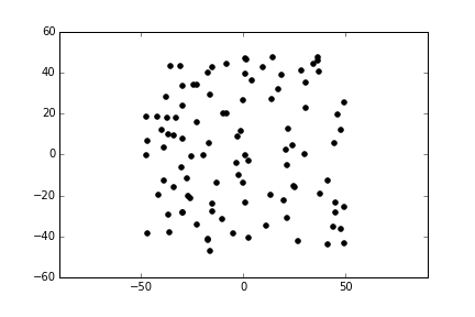
Imagine that you have a system with open boundaries in two dimensions, with N=100 particles.

Our goal is to compute the forces (it doesn’t matter what sort of force) between all these particles at a given time step. With the forces, we can calculate their accelerations, from which we obtain velocities and then their displacements. The displacements will tell us their positions in the next time step. We use this to compute the forces and the cycle goes on, for some period of time.

Assuming that these forces are functions of distances, we need to compute the distance between all permutations of particles. We can construct a matrix of distances, which will look like this:

\[ \begin{pmatrix} d_{1,1} & d_{1,2} & .. & d_{1,N} \
d_{2,1} & d_{2,2} & .. & d_{2,N} \
.. & .. & .. & .. \
d_{N,1} & d_{N,2} & .. & d_{N,N} \
\end{pmatrix} \]

We must generate the initial positions of 100 particles, and construct the distance matrix:

import numpy as np

L   = 100       # simulation box dimension
N   = 100       # Number of particles
dim = 2         # Dimensions

# Generate random positions of particles
r = (np.random.random(size=(N,dim))-0.5)*L

# Compute distance matrix
D = np.zeros(shape=(N,N), dtype=float)

# This is the N-squared operation
for i in range(N):
    for j in range(N):
        dr = r[j]-r[i]                  # difference between 2 positions
        D[i,j] = np.sqrt(sum(dr*dr))    # calculate distance and store

print(D[:3,:3])                         # print small section of the matrix

>>> [[  0.          14.47476649  68.4285819 ]
    [ 14.47476649   0.          53.99224333]
    [ 68.4285819   53.99224333   0.        ]]

Upper Triangular Distance Matrix

For 100 particles, in this algorithm, we are making 10,000 distance calculations. We can do better. Firstly, notice that the diagonal values are zero. The distance of a particle with itself is always obviously zero. Secondly, the matrix is symmetric i.e. reversing the order of indices does not affect the calculated distance. So we are computing distances between particle pairs twice, when we can get away with half the number of calculations. All we need to do is compute the upper triangular matrix of D. The N-squared operation will then become:

Code 1

# This is the N-squared operation
for i in range(N):
    for j in range(i+1,N):              # j>i (second index is always greater than first)
        dr = r[j]-r[i]                  # difference between 2 positions
        D[i,j] = np.sqrt(sum(dr*dr))    # calculate distance and store

We have now decreased the number of calculations to 4,950. In terms of the algorithm, there isn’t much more that we can do. However, we can do a lot better if we learn some pythonic tricks.

• Perform expensive numpy functions such as, np.sqrt, as few times as possible. For instance, the solution will be identical, if we take the square root of the matrix, after the squared distances are calculated.
• Avoid explicit for loops, when possible. They are usually rather slow in Python. If you find a way to offload looping duties to Python implicity, you will generally get much more readable and faster code. Namely, if the body of your loop is simple, as it is here, the interpreter of the for loop itself contributes substantially to the overhead.
• Reduce data access. So far, we created an array of zeros, and updated their values by accessing them. This is inefficient.

With these three things in mind, let’s do better! For this we need to learn a neat numpy function called np.triu_indices. This gives the upper triangular matrix indices i.e. exactly the same indices that we were generating using our range function in a for loop.

Code 2

import numpy as np

L   = 100       # simulation box dimension
N   = 100       # Number of particles
dim = 2         # Dimensions

# Generate random positions of particles
r = (np.random.random(size=(N,dim))-0.5)*L

# uti is a list of two (1-D) numpy arrays  
# containing the indices of the upper triangular matrix
uti = np.triu_indices(N,k=1)        # k=1 eliminates diagonal indices

# uti[0] is i, and uti[1] is j from the previous example
dr = r[uti[0]] - r[uti[1]]            # computes differences between particle positions
D = np.sqrt(np.sum(dr*dr, axis=1))    # computes distances; D is a 4950 x 1 np array

We have done in three lines, what we previously achieved in five, and we have no more for loops. Timing them on my computer shows the gulf of performance between the two approaches, for a 1000 particles system: Code 1 takes around 3.4 seconds, and Code 2 takes around 0.0005 seconds. Perhaps you noticed that I did cheat a little by not generating a NxN matrix, as in Code 1. But even recasting the values using scipy.spatial.distance.squareform into a NxN matrix does not slow the code significantly.

The easiest method to solve this problem, as I mentined earlier, is to use the scipy.spatial.distance.pdist function. Its a one-liner:

Code 3

import numpy as np
from scipy.spatial.distance import pdist

L   = 100       # simulation box dimension
N   = 100       # Number of particles
dim = 2         # Dimensions

# Generate random positions of particles
r = (np.random.random(size=(N,dim))-0.5)*L
D = pdist(r)

This was, to my surprise, not as fast as Code 2.

Particles within periodic boundaries

In molecular dynamics, we frequently encounter periodic boundaries. It is the case a large (infinite) system is approximated by using a small part called a unit cell. The geometry of the unit cell is tiled such that when an object passes through one side of the unit cell, it re-appears on the opposite side with the same velocity.

A decision must be made, here. Do we

• “fold” particles into the simulation box when they leave it, or
• do we let them go on, and wander out of the unit cell, but compute interactions with the nearest images when necessary?

Wrapped

In the first approach, where the positions of particles are wrapped, they are necessarily within the unit cell. Restricting the coordinates within the unit cell is easy. If x is the position of the particle in some arbitrary dimension, and L is the length of the box in that dimension, the approach can be described by the following C++ code:

if (x <  -L * 0.5) x = x + L
if (x >=  L * 0.5) x = x - L

Naively computing distances between particle pairs will omit pairs where one particle is close to the boundary and its counterpart is lurking in the adjacent cell. Distances and vectors between objects should obey, what is known as the minimum image criterion. And we can calculate the minimum image distance in the following manner:

dx = x[j] - x[i]
if (dx >   L * 0.5) dx = dx - L
if (dx <= -L * 0.5) dx = dx + L

Obviously, this needs to be repeated for the number of dimensions that the particles exist in. In Python, these codes will look like this:

L   = 100       # simulation box dimension
N   = 100       # Number of particles
dim = 2         # Dimensions

# Particles have purposely wandered out of L
r = (np.random.random(size=(N,dim))-0.5)*1.5*L

# Wrapping step
r[r  < -L*0.5] += L
r[r >=  L*0.5] -= L

# Distance calculation step
uti = np.triu_indices(N, k=1)        

# uti[0] is i, and uti[1] is j from the previous example
dr = r[uti[0]] - r[uti[1]]            # computes differences between particle positions

# Minimum image convention
dr[r >   L*0.5] -= L                
dr[r <= -L*0.5] += L
D = np.sqrt(np.sum(dr*dr, axis=1))    # computes distances; D is a 4950 x 1 np array

Unwrapped

Given the size of the box, we can also directly compute the distances according to the minimum image convention, without wrapping the particles within the unit cell. This is done here in C++ in the following manner:

L_r = 1.0 / L;        // L is the box length

dx = x[j] - x[i];     // Compute distance between particle i and j
dx -= x_size * nearbyint(dx * L_r);

In Python:

r = (np.random.random(size=(N,dim))-0.5)*1.5*L
uti = np.triu_indices(N, k=1)        
dr = r[uti[0]] - r[uti[1]]

# Minimum image distance of unwrapped dr
dr -= L * np.round(dr/L)

Bottom line

Even though Python is a high level language, we can get a lot of traction in molecular dynamics, even for a relatively large number of particles. I prefer to perform my analysis in Python, because the code is readable and easy to debug in the future. The issue of N-squared time complexity, still remains, in this algorithm, but is greatly alleviated by more pythonic coding.